Into to Partitioning or Sharding

Introduction

For very large datasets, or very high query throughput, replication is not sufficient: we need to break the data into partitions, also known as sharding! Each partition can be stored on a separate physical device, potentially across different locations, allowing for better resource utilization and faster access times.

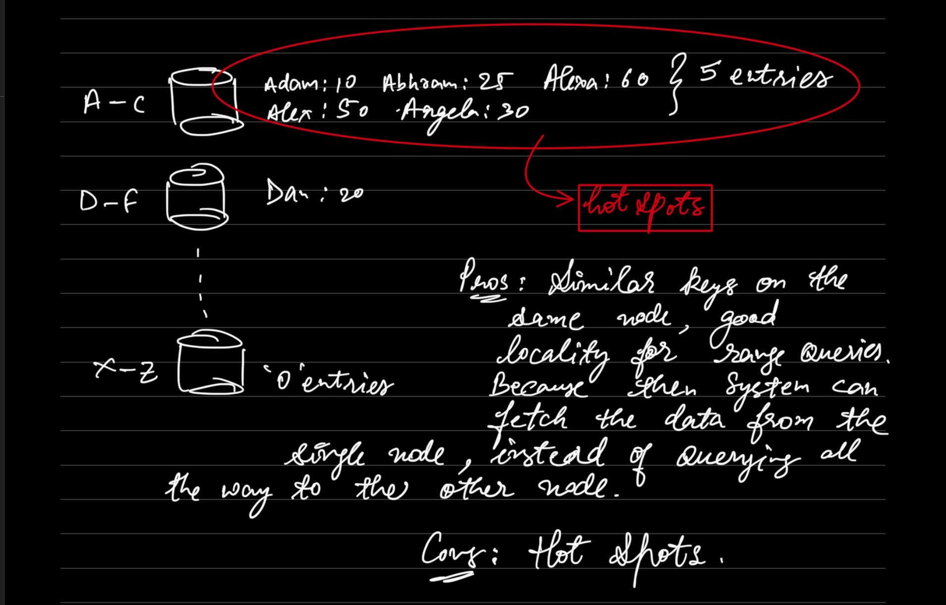
Our goal with partitioning is to spread the data and the query load evenly across the nodes. If partitioning is unfair, so that some partitions have more data or queries than others, we call it skewed. In extreme, case all the load could end up on one partition, so 9 out of 10 nodes are idle and your bottleneck is the single busy node. A partition with disproportionately high load is called hot spot.

We can avoid hotspots with various partitioning techniques:

1. Range Based Partitioning (Key Range Partitioning)

Assign continuous range of keys (from some minimum to some maximum) to each partition. If you also know which partition is assigned to which Node, then you can make your request directly to the appropriate node (or, in the case of encyclopedia, pick the correct book off the shelf).

The ranges of the keys might not be evenly spaced, because your data might not be evenly distributed. For example, in Figure 6-2, volume 1 contains words starting with A and B, but volume 12 contains words starting with T, U, V, X, Y, and Z. Simply having one volume per two letters of the alphabet would lead to some volumes being much bigger than others.

[! note] Used in: Bigtable, HBase, Rethink, and MongoDB before version 2.4.

Within each partition we can keep the keys sorted (SSTables and LSM Trees). $O(logN)$ scans.

Cons:

• HotSpots

2. Hash Based Partitioning(Hashing a key) - Consistent Hashing

This technique is used to evenly distribute data across a distributed system by hashing keys to determine their partition. This approach is effective in preventing single nodes from becoming a bottleneck under typical conditions.

Note

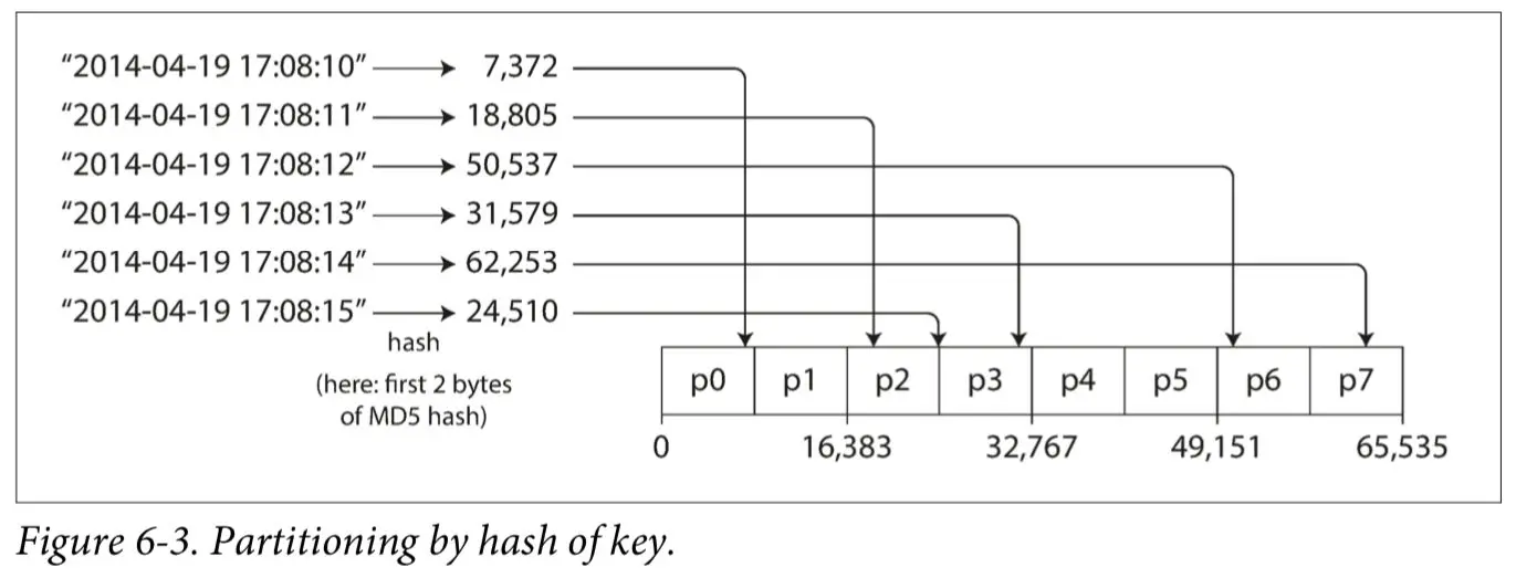
For partitioning purposes, the hash function need not be cryptographically strong: for example, Cassandra and MongoDB use MD5, and Voldemort uses the Fowler– Noll–Vo function. Many programming languages have simple hash functions built in (as they are used for hash tables), but they may not be suitable for partitioning: for example, in Java’s Object.hashCode() and Ruby’s Object#hash, the same key may have a different hash value in different processes

Once you have a suitable hash function for keys, you can assign each partition a range of hashes (rather than a range of keys), and every key whose hash falls within a partition’s range will be stored in that partition.

Pros: Relatively even distribution of keys, less hot spots! Cons: No data locality for range queries.

Hash-based partitioning can scatter adjacent keys across all partitions, making efficient range queries difficult. In MongoDB’s hash-based sharding mode, range queries need to be sent to all partitions. Range queries on primary keys are NOT supported by Riak, Couchbase, or Voldemort. Cassandra offers a compromise by allowing tables to have compound primary keys. The first part of the key is hashed for partitioning, while the remaining columns are used as concatenated index for sorting the data in Casandra’s SSTables. This allows efficient range scans if a fixed value is provided for the first part of the key. The concatenated index approach enables an elegant data model for one-to-many relationships. For example, on a social media site, one user may post many updates. If the primary key for updates is chosen to be (user_id, update_timestamp), then you can efficiently retrieve all updates made by a particular user within some time interval, sorted by timestamp. Different users may be stored on different partitions, but within each user, the updates are stored ordered by timestamp on a single partition.

3. Partitioning & Secondary Indexes

A secondary index usually doesn’t identify a record uniquely but rather is a way of searching for occurrences of a particular value: find all actions by user 123, find all articles containing the word hogwash, find all cars whose color is red, and so on. Secondary indexes are essential in relational databases and are also widely used in document databases. Although many key-value stores like HBase and Voldemort initially avoided implementing secondary indexes due to their complexity, some, like Riak, have started to include them due to their utility in data modeling. Additionally, secondary indexes are a fundamental feature of search servers like Solr and Elasticsearch, which rely on them heavily for efficient querying.

3.1 Partitioning Secondary Indexes by Document (Local Secondary Index)

Users want to buy the car? Imagine each listing has a unique ID - call it the document ID - and you partition the database by the document ID (for example: IDs $0$ to $499$ in partition $0$, IDs $500$ to $999$ in partition $1$, etc.). Search by color and make? Declare the index, the db can perform the indexing automatically. For example: whenever a red car is added to the database, the database partition automatically adds it to the list of document IDs for the index entry $color:red$.

Note

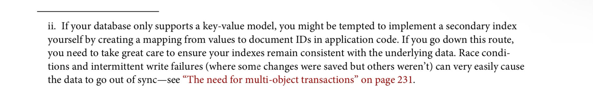
Race conditions can occur when multiple operations need to be performed in a sequence, but there’s a possibility that the operations might be interrupted or interleaved by other operations. In the context of implementing a secondary index in a key-value database, the race condition can happen as follows:

1. Concurrent Writes: If two or more processes are writing to the database simultaneously, one process might update the primary data while another updates the index. If these updates are not coordinated, the index can become inconsistent with the primary data.
2. Intermittent Failures: If an update to the primary data succeeds but the corresponding update to the index fails (or vice versa), the index will not accurately reflect the data. This can occur due to network issues, crashes, or other system failures.
3. Lack of Atomicity: Without atomic multi-object transactions, there is no guarantee that changes to both the primary data and the index will either both complete or both fail. This partial completion can leave the database in an inconsistent state.

For example, consider an operation that updates a user’s email address in both the primary data store and a secondary index. If the email update in the primary store succeeds but the update in the secondary index fails, the secondary index will not reflect the user’s current email address. Subsequent operations that rely on the secondary index may then operate on outdated or incorrect information.

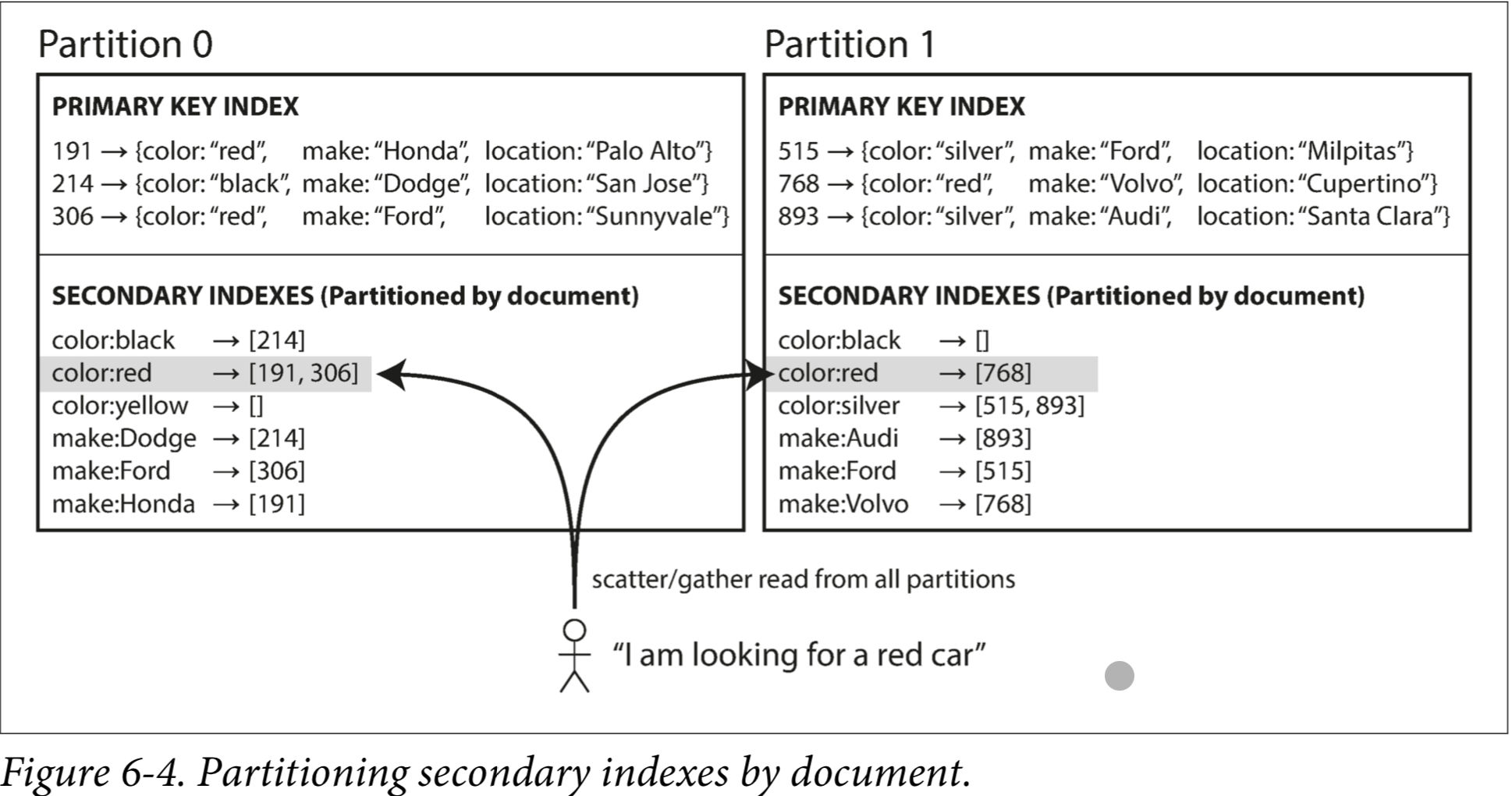
Each partition is completely separate: each partition maintains its own secondary indexes, covering only the documents in that partition. Whenever you need to write to the database—to add, remove, or update a document—you only need to deal with the partition that contains the document ID that you are writing. Hence, known as local index.

Con:

If you want to search for red cars, you need to send the query to all partitions, and combine all the results you get back. This approach of executing queries across multiple partitions and then aggregating the results is known as scatter gather. Ultimately we’ll need to deal with data consistency issues, network latency issues, etc. It’s not always possible to partition the data such that secondary index queries can be served from a single partition. Nevertheless it’s used in: MongoDB, Riak, Cassandra, Elasticsearch, Solr Cloud & VoltDB.

3.2 Partitioning Secondary Indexes by Term (Global Index)

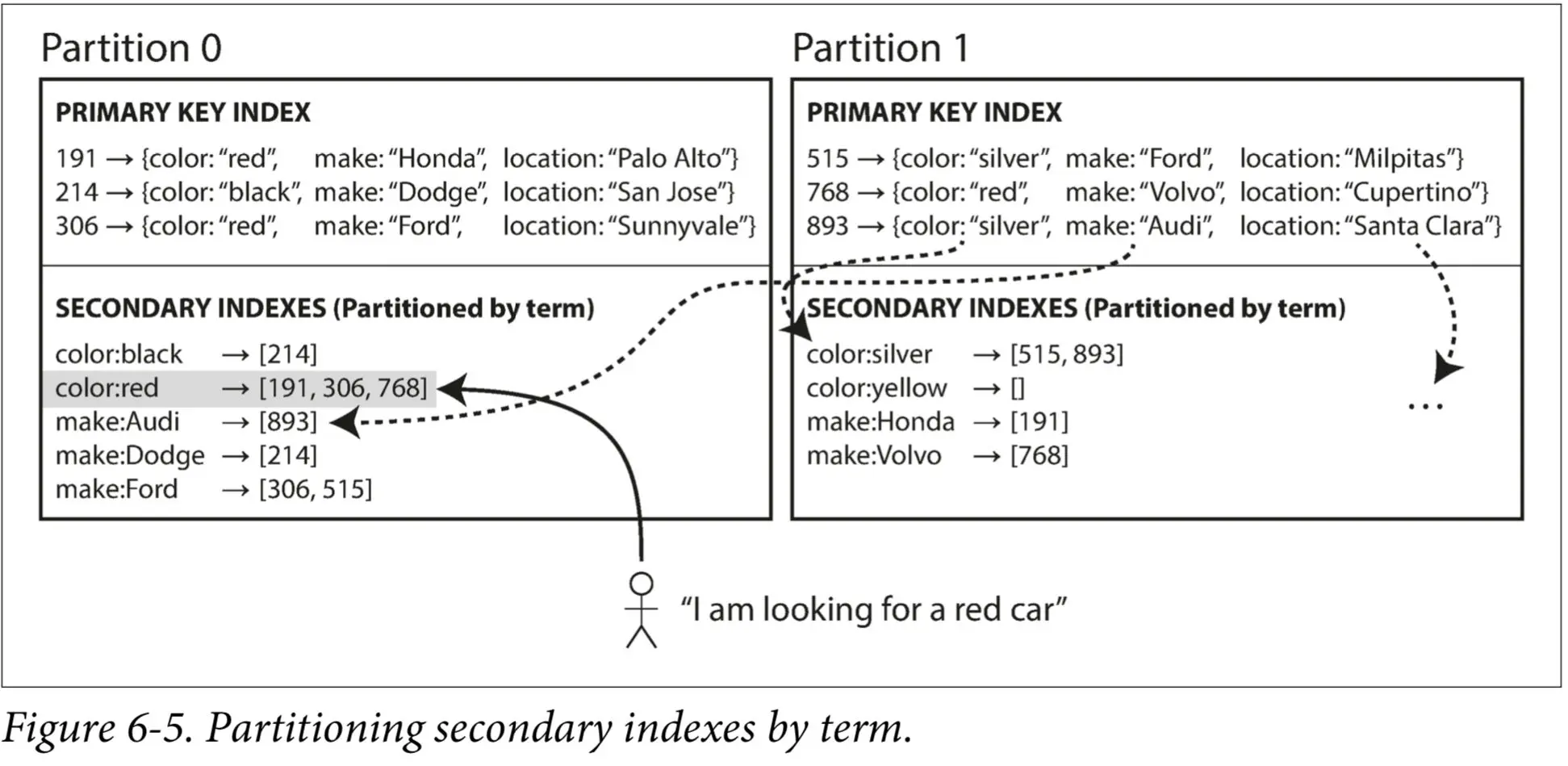
Partitioning Secondary Indexes by Term, also known as term-based partitioning, is a method used to distribute the secondary indexes of a database across multiple partitions to improve the efficiency of read operations.

Note

• For example, Amazon DynamoDB states that its global secon‐dary indexes are updated within a fraction of a second in normal circumstances, but may experience longer propagation delays in cases of faults in the infrastructure.
• Other uses of global term-partitioned indexes include Riak’s search feature and the Oracle data warehouse, which lets you choose between local and global indexing

How It Works:

1. Term-Based Partitioning:

   • In a global index, the index entries (terms) are partitioned. For instance, if the secondary index is on car colors, all red cars from different partitions are indexed under color:red. This index is then partitioned further. For example, colors starting with letters a to r might be in one partition, while those from s to z are in another.

2. Advantages:

   • Efficient Reads: Unlike local indexes, which require scatter/gather queries across all partitions, a global index allows the client to query only the partition containing the desired term, significantly reducing query complexity and improving performance.
   • Centralized Index: By consolidating the index entries, it ensures that the look-up for a specific term is streamlined to a specific partition.

3. Challenges:

   • Write Complexity: Writing data becomes more complex because a single document might update multiple partitions of the index. For example, a document with multiple terms (like a car with multiple attributes) could affect several index partitions.
   • Rebalancing: Managing and rebalancing the partitions of the global index, especially as data grows and nodes are added or removed, can be challenging. Techniques like dynamic partitioning or proportional partitioning to nodes are used to address these challenges.

Example: Consider a database managing a large number of documents, such as a used car listing site. Each listing includes attributes like color and make. If the secondary index on color is term-partitioned:

• Local Index: Each partition has its own secondary index. To find all red cars, you would need to query each partition.
• Global Index: All red cars are indexed together, and the index is partitioned, say alphabetically by color. Queries for red cars are directed to the specific partition holding the color:red index.

Con:

• Increased Write Complexity: When a document is written or updated, it may affect multiple partitions of the global index, requiring coordinated updates across those partitions. This can lead to more complex and slower write operations.
• Coordination Overhead: Managing a global index requires more coordination between partitions, especially to maintain consistency and integrity of the index. This can introduce additional overhead and complexity in the system.
• Increased Latency for Write Operations: Because writes may need to update multiple index partitions, the latency for write operations can increase. This is especially problematic in systems with high write loads.

Handling write failures in systems with term-based partitioned secondary indexes involves trade-offs between consistency, performance, and complexity. Techniques such as two-phase commit, compensating transactions, and eventual consistency are commonly used to manage these challenges, each with its own advantages and limitations.

Handling Write Failures During Multi-Node Updates

1. Atomicity and Transaction Support:
   • Two-Phase Commit (2PC):
     • To ensure atomicity (all-or-nothing) in distributed systems, a two-phase commit protocol can be used.
     • In the first phase, all nodes prepare for the write and report back if they are ready to commit.
     • In the second phase, the coordinator either commits or aborts the transaction based on the responses. However, 2PC introduces additional latency and can be a bottleneck.
   • Distributed Transactions: Some databases support distributed transactions, which ensure that all parts of the transaction either commit or roll back together. This helps maintain consistency but can reduce performance due to the overhead of managing transactions across nodes.
2. Compensating Transactions:
   • Compensating actions are designed to reverse the changes made by the original transaction steps.
   • If a write operation fails after partially updating some nodes, compensating transactions can be used to roll back the changes made to the nodes that were successfully updated. This helps maintain consistency but requires additional logic to manage the rollbacks.
3. Eventual Consistency:
   • Some systems opt for eventual consistency, where writes are propagated to all nodes asynchronously. If a write fails, the system eventually reconciles the inconsistencies. This approach improves write performance but may lead to temporary inconsistencies .
4. Retry Mechanism:
   • Implementing a retry mechanism can help recover from transient failures. The system can retry the write operation a certain number of times before aborting. This is simple to implement but might not be suitable for persistent failures.